TUESDAY, APRIL 26, 2011
libsvm
- Collect Training Data: (with your own codes to create TrainingData)
- Scale training data:
- Get parameters and Train data with parameters
- Test/Run classificaiton: same way to get test data:
fprintf(fp, "3 "); // label: 1, 2 ...
for (j = 0; j < 12; j++)
fprintf(fp, "%d:%f ", j, mel_cep[j]);
fprintf(fp, "\n");
svm-scale.exe -l -1 -u 1 -s range1 TrainingData > TrainingData.scale
python gird.py TrainingData.scaleGot the best parameters c, g (2.0, 2.0)
svm-train.exe -c 2 -g 2 TrainingData.scale
The output is TrainingData.scale.model
//fprintf(fp, "1 "); // if you know the label, can get the accuracy output with this
for (j = 0; j < 12; j++)
fprintf(fp, "%d:%f ", j, mel_cep[j]);
fprintf(fp, "\n");
Scale the test data with the same scaling factor with training data:
svm-scale.exe -r range1 test_libsvm.t > test_libsvm.t.scaleRun the classification/Prediction: (write your own codes here)
svm-predict.exe test_libsvm.t.scale TrainingData.scale.model test_libsvm.t.predict
===================
To use the cross validation to check the accuracy:
svm-train.exe -v 5 TrainingData
svm-train.exe -v 5 TrainingData.scale
svm-train.exe -c 2 -g 2 -v 5 TrainingData.scale
without normalize (scale), Cross Validation Accuracy = 87%
with scale (-1 1), Cross Validation Accuracy = 92%
with parameter selection –c 2 –g 2, Cross Validation Accuracy = 95%
To get the probability information, in training part, use:
svm-train.exe -c 2 -g 2 -b 1 TrainingData.scale
In test/run part, make "int predict_probability=1;" and the program will call "predict_label = svm_predict_probability(model,x,prob_estimates);" , which writes the probability value in the output file.
THURSDAY, JANUARY 27, 2011
WDL example for Reaper
- download WDL library at this link
- Open the Example project under IPlug, and add a new project such as ‘classify’
- Configuration Properties General: Type: Dynamic Library (.dll)
- Configuration Properties Debugging: if you want to use Reaper
- C++-Addi Include Dir: ..\IPlug;..\..\wdl\lice;..\VST_aSDK\vstsdk2.4\pluginterfaces\vst2.x
- C++ – Prep Definitions: VST_API;WIN32;_WIN32_WINNT=0x0501;WINVER=0x0501;_CRT_SECURE_NO_DEPRECATE;_DEBUG
- C++ – Code Generation – Runtime Lib: Multi-threaded Debug(/MTd)
- Linker – General – Output File: $(OutDir)/$(ProjectName)_DEBUG.dll
- Linker – General –Enable Incremental linking: Yes (/Inc)
- Linker – General –Addi Library DIr: "..\..\IPlug\$(ConfigurationName)";"..\..\lice\$(ConfigurationName)"
- Linker – Input – Addi Depend.:shell32.lib lice.lib IPlug.lib user32.lib gdi32.lib comdlg32.lib
- Linker – Debugging – Generate prog Database File:$(OutDir)/test.pdb
- Linker – SYstem – subsys: Windows (/SUBSYSTEM:WINDOWS)
- Linker – Advanced – maybe
WEDNESDAY, JANUARY 26, 2011
Basic steps of audio source localization
- Bandpass filter input signals (300Hz~6KHz) of every channel
- For first winSize samples, use as noise samples. (for compensation use)
- Use Hann window to taper every winSize input signals
- Find the peak value and its channel number
- Use Hilbert Transform to that channel and find the peak location
- shift back some samples and get the processing window which includes the peak signal.
- Whiten the window signals
- for every pixel, get the weight value for every channel and delay the signals of most channels
- calculate the Steered Response Coherent Power for ever pixel. Coherent power differs from regular power which squared sum normalized by time. In coherent power, only the power from signal cross correlation between two channels is used in the summation. (x1[i]+…xN[i])^2 - (x1[i]^2+…xN[i]^2). where xn[i] is delayed signal of one channel. Large positive value of SRCP indicates a strong correlation or coincidence between signals in different channels.
FRIDAY, JANUARY 14, 2011
Read .wav file in C
Use the open source library:
http://www.mega-nerd.com/libsndfile/
In project properties: C/C++ Additional Include Directories: "C:\Program Files\Mega-Nerd\libsndfile\include"
Linker Additional Library Directories: C:\Program Files\Mega-Nerd\libsndfile
Input Additional Dependencies: libsndfile-1.lib
http://www.mega-nerd.com/libsndfile/
In project properties: C/C++ Additional Include Directories: "C:\Program Files\Mega-Nerd\libsndfile\include"
Linker Additional Library Directories: C:\Program Files\Mega-Nerd\libsndfile
Input Additional Dependencies: libsndfile-1.lib
#include <sndfile.h>
int _tmain(int argc, _TCHAR* argv[])
{
    float buf [1024] ;
    int i;

    SF_INFO sfinfo;
    sfinfo.samplerate = 44100;
    sfinfo.channels = 1;
    sfinfo.format = 0;

    SNDFILE* sndfile =  sf_open("C:\\clap1mic1.wav", SFM_READ, &sfinfo) ;
    if (sndfile == NULL)
        printf("NULL\n");
    sf_count_t  s_len = sf_read_float(sndfile, buf, 1024);

    for (i = 0; i < s_len; i++)
        printf("%f\n", buf[i]);

    sf_close(sndfile);
    return 0 ;
}
TUESDAY, FEBRUARY 23, 2010
TUESDAY, FEBRUARY 16, 2010
Spectral Centroid in Audio
The center of mass of the spectrum.

x(n) is the magnitude of bin number, f(n) is the center frequency of that bin. The following MATLAB function is from the exchange website;
x(n) is the magnitude of bin number, f(n) is the center frequency of that bin. The following MATLAB function is from the exchange website;
function C = SpectralCentroid(signal,windowLength, step, fs)
signal = signal / max(abs(signal));
curPos = 1;
L = length(signal);
numOfFrames = floor((L-windowLength)/step) + 1;
H = hamming(windowLength);
m = ((fs/(2*windowLength))*[1:windowLength])';
C = zeros(numOfFrames,1);
for (i=1:numOfFrames)
    window = H.*(signal(curPos:curPos+windowLength-1));
    FFT = (abs(fft(window,2*windowLength)));
    FFT = FFT(1:windowLength);
    FFT = FFT / max(FFT);
    C(i) = sum(m.*FFT)/sum(FFT);
    if (sum(window.^2)<0.010)
        C(i) = 0.0;
    end
    curPos = curPos + step;
end
C = C / (fs/2);
MONDAY, FEBRUARY 15, 2010
Mel-frequency cepstrum coefficients (mfcc) in audio
The word 'cepstrum' reverses the first 4 letters of 'spectrum', it takes Fourier transform to the decibel of spectrum. The process is:
signal -> FFT -> abs()&square -> log -> FFT -> abs()&square -> spectrum
MFCC is a nonlinear "spectrum-of-a-spectrum". It represents the short-term power spectrum of a sound.
The MFCC procedure is:
audio signal -> FFT -> map to mel scale -> log -> DCT -> MFCC (the amplitudes of the result spectrum)
The matlab code of MFCC is in following links: link0, link1, link2,Auditory Toolbox
MONDAY, DECEMBER 14, 2009
Spectral Flux (SF) in Audio
Also called Spectral Variation. Spectral flux measures how quickly the power spectrum changes. Spectral flux is defined as the variation value of spectrum between the adjacent two frames in a short-time analyze window. Spectral flux can be used to determine the timbre of an audio signal. The MATLAB code:
[wav fs] = wavread('DEMO.wav');
wav = wav / max(max(wav));
window_length = 2 * fs; % assume the windows is 2 seconds
step = 1 * fs;          % and it has overlap in windows
frame_num = floor((length(wav)-window_length)/step) + 1;

H = hamming(window_length);
flux = zeros(frame_num, 1);
pos = 1;
FFT_prev = 0;

for i=1:frame_num
  wav_window = H .* wav(pos:pos + window_length-1);
  FFT = abs(fft(wav_window, 2*window_length));
  FFT = FFT(1 : window_length);
  FFT = FFT/max(FFT);

  flux(i) = sum((FFT - FFT_prev) .^ 2);
  FFT_prev = FFT;
  pos = pos + step;
end
Audio features in two levels
Audio features are usually extracted in two levels: short term (frame) level, and long term (clip) level.
A frame is defined as a group of neighboring samples which last about 10-40ms, assume the audio signal is stationary and short-term features such as energy and Fourier transform coefficients can be extracted.
For a feature to reveal the semantic meaning, we use from one second to several tens seconds audio clips, sometimes called ‘window’.
THURSDAY, OCTOBER 29, 2009
Zero Crossing Rate (ZCR) in Audio
ZCR is a very useful audio feature, it is defined as the number of times that the audio waveform crosses the zero axis.

fs is the sampling rate. ZCR is used to discern unvoiced speech. Usually unvoiced speech has a low short-term energy but a high zero crossing rate. Combining ZCR and STE to prevent low energy unvoiced speech frames from being classified as silent. MATLAB code:

fs is the sampling rate. ZCR is used to discern unvoiced speech. Usually unvoiced speech has a low short-term energy but a high zero crossing rate. Combining ZCR and STE to prevent low energy unvoiced speech frames from being classified as silent. MATLAB code:
% assume the window size is 2 seconds
% there are overlaps in windowing
% assume the step of shif is 1 second

[wav fs] = wavread('DEMO.wav');
wav = wav / max(max(wav));
window_length = 2 * fs;
step = 1 * fs;
frame_num = floor((length(wav)-window_length)/step) + 1;

zcr_ = zeros(frame_num, 1);
wav_window2 = zeros(window_length, 1);
pos = 1;

for i=1:frame_num
   wav_window = wav(pos:pos + window_length-1);
   wav_window2(2:end) = wav_window(1:end-1);
   zcr_(i) = 1/2 * sum(abs(sign(wav_window) - ...
       sign(wav_window2))) * fs / window_length;
   pos = pos + step;
end
WEDNESDAY, OCTOBER 28, 2009
Short-Time Energy (STE) in Audio
STE is the audio feature that is widely used and the easiest. It is also called volume. STE is a reliable indicator for silence detection. Normally STE is approximated by the rms (root mean square) of the signal magnitude within each frame. The MATLAB code:
The short time energy of audio signal depends on the gain value of the recording devices. Usually we normalize the value for each frame
% assume the window size is 2 seconds
% there are overlaps in windowing
% assume the step of shif is 1 second

[wav fs] = wavread('DEMO.wav');
wav = wav / max(max(wav));
window_length = 2 * fs;
step = 1 * fs; % has overlap
frame_num = floor((length(wav)-window_length)/step) + 1;

energy = zeros(frame_num, 1);
pos = 1;

for i=1:frame_num
   wav_window = wav(pos:pos + window_length-1);
   energy(i) = 1/window_length * sum(wav_window.^2);
   pos = pos + step;
end
MONDAY, OCTOBER 26, 2009
Write audio data to a GIF file to display animation
Sometimes it can be applied in the PPT presentation.
In the following MATLAB code, the framerate is 20frame/second, the window size for audio data is 2 seconds, and no overlap. It basically saves the ‘plot’ figures to a GIF frame by frame:
In the following MATLAB code, the framerate is 20frame/second, the window size for audio data is 2 seconds, and no overlap. It basically saves the ‘plot’ figures to a GIF frame by frame:
[wav, fs] = wavread('DEMO.wav');
window_length = 2; %2 seconds
window_sample = window_length * fs;
for i = 1 : window_sample : length(wav)-window_sample
block = wav(i:i+window_sample);
time = (0:1/fs:(length(block)-1)/fs) + i/fs;
h = plot(time, block);
axis([time(1) time(end) -1 1]);saveas(gcf, 'block.jpg');
img_block = imread('block.jpg');
[ind, map] = rgb2ind(img_block,256);
if i == 1
writemode = 'overwrite';
else
writemode = 'append';
end
imwrite(ind,map,'WaveGIF.gif','gif', ...
'DelayTime', 1/20, 'WriteMode',writemode);
end
THURSDAY, OCTOBER 22, 2009
Compute windowed block FFT of audio data
When we start to process the audio data, we cut it to a lot of blocks. There are some overlaps between blocks. If we know the size of a block and how blocks overlap, we can get the total block number and the block information (start and end information). MATLAB code:
If we want to get the FFT of windowed blocks,
% wav is the audio data
% blocksize, let's say 1024
% n: if = 16, means 16 blocks overlap together
% that right-shifts pretty slowly
% blocks: start/end of every block
% ex: blocks(1)=1, blocks(2)=65, blocks(3)=129

function blocks = wavblocks(wav, blocksize, n)

blocks_num = floor((length(wav)/blocksize-1)*n);
blocks = floor((0:blocks_num)*(blocksize/n)+1);
blocks = wavblocks(snd, windowsize, overlap);
numblocks = length(blocks);

minfreq = 200; %specific freq range
maxfreq = 20000;
fs = 8000; % sampling rate

% block2fft func is in last post, snd is audio data
% t is the fft power of a block within specific freq range
t = length(block2fft(snd(blocks(1) : blocks(1) + windowsize - 1),
  fs, minfreq, maxfreq));
p = zeros(tl, numblocks);

hann_window(1:windowsize, 1) = 0.54 + 0.46*
         cos(2*pi*(0:windowsize-1)/(windowsize-1));

%p(:,i) is the fft power of a windowed block
for (i = 1:numblocks)
p(:, i) = block2fft(snd(blocks(i) : blocks(i) + windowsize
          - 1).*hann_window', fs, minfreq, maxfreq);
end
WEDNESDAY, OCTOBER 21, 2009
Calculate the power of audio in frequency block
Here is the matlab code, it shows the power between frequency 200-2000. This is the power of all audio data instead of a small window block (like 256 samples):
The x-axis is plotting the number of samples. It is more useful to plot the single-sided spectrum with frequency in x-axis. For example, we want to display 200-9000Hz spectrum:
>> [snd samplefreq] = wavread('crash.wav');
>> num_samples = length(snd);
>> minfreq = 200; maxfreq = 2000;
>> f = fft(snd) / (num_samples/2);
>> seconds = num_samples / samplefreq;
>> low = floor(seconds * minfreq);
>> high = floor (seconds * maxfreq);
>> p = abs(f(low:high)) .^ 2;
>> figure; plot(p);
If you want to show the fft result directly, use ‘fftshift’ to produce a more standard plot with the low frequencies in the center of plot:plot(abs(f)); plot(abs(fftshift(f)));
Ns = length(p);
plot([201:2*(9000-200)/Ns:9000],p(1:Ns/2-1)); %make sure the size are the same
TUESDAY, SEPTEMBER 29, 2009
TUESDAY, SEPTEMBER 22, 2009
Basic audio analysis methods
1. Zero-crossing rate: the number of crossings per second will equal twice the frequency. Threshold crossing rate: count only when signal drops below the threshold
2. Frame power: sum(segment .^ 2)/length(segment);
3. Average magnitude difference: sum(abs(segment)) / length(segment);
4. Spectral measures: ratio = high_freq / low_freq
5. Cepstral analysis: it is the inverse FFT of the logarithm of FFT (cceps, iccesp in Matlab)
2. Frame power: sum(segment .^ 2)/length(segment);
3. Average magnitude difference: sum(abs(segment)) / length(segment);
4. Spectral measures: ratio = high_freq / low_freq
5. Cepstral analysis: it is the inverse FFT of the logarithm of FFT (cceps, iccesp in Matlab)
FRIDAY, SEPTEMBER 18, 2009
Audio Segmentation: overlap, windowing, filtering
Overlap: 25% and 50% overlaps are common. A regular process is:
A single FFT can trade off between higher frequency resolution (more samples) or higher time resolution (fewer samples), but cannot do both simultaneously.
Windowing:
The windowed DFT is the product of the original signal and the windowing function: x[n] is a signal of infinite extend, n is the sample index, g[n] is a finite window

In frequency domain this is a convolution with the window DFT:

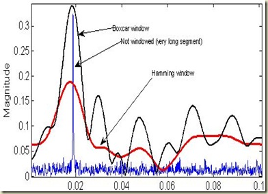
Here is the impact of windowing:
Spectrogram:
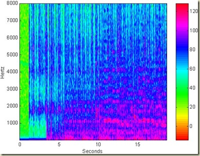
Short-time Fourier transform (STFT) is a sliding-window narrow Fourier transform that is repeated sequentially over a long vector of samples. A spectrogram is essentially a set of STFT plotted as frequency against time with the intensity (z-axis) given as a grey scale, or color pixel.
The horizontal axis of an FFT plot is traditionally used to represent frequency, and the vertical axis would display amplitude. A spectrogram plots time along the horizontal axis, frequency on the vertical and amplitude on the z-axis (as color or grey scale).
Filters:
Filters are designed based on specifications given by:
- segment into 50% overlapped frames
- window each frame (ex Hamming window, blackman window)
- add overlaps to reconstruct
A single FFT can trade off between higher frequency resolution (more samples) or higher time resolution (fewer samples), but cannot do both simultaneously.
Windowing:
The windowed DFT is the product of the original signal and the windowing function: x[n] is a signal of infinite extend, n is the sample index, g[n] is a finite window
In frequency domain this is a convolution with the window DFT:

Here is the impact of windowing:

Spectrogram:
Short-time Fourier transform (STFT) is a sliding-window narrow Fourier transform that is repeated sequentially over a long vector of samples. A spectrogram is essentially a set of STFT plotted as frequency against time with the intensity (z-axis) given as a grey scale, or color pixel.
The horizontal axis of an FFT plot is traditionally used to represent frequency, and the vertical axis would display amplitude. A spectrogram plots time along the horizontal axis, frequency on the vertical and amplitude on the z-axis (as color or grey scale).

Filters:
Filters are designed based on specifications given by:
- spectral magnitude emphasis
- delay and phase properties through the group delay and phase spectrum
- implementation and computational structures
- (IIR) besself, butter, cheby1, cheby2, ellip, prony, stmcb
- (FIR) fir1, fir2, kaiserord, firls, firpm, firpmord, fircls, fircls1, cremez
- (Implementation) filter, filtfilt, dfilt
- (Analysis) freqz, FDAtool, SPtool
Matlab: Sound generation
Pure tone: unmodulated sinusoid, matlab function:
Generate sound with different frequency:
% Ft: frequency of the tone
% Fs: sample rate
% Td: last seconds
% Output is a row vector s containing the sampled point
% t is an optional and is the time axis associated with s

function [s, t] = tonegen(Ft, Fs, Td)
t = [1:Fs*Td]/Fs;
s = sin (2 * pi * t * Ft);

% example:
y = tongen(440, 16000, 5);
soundsc(y, 16000);
% frc: time-varying frequency
% Fs: sample rate

function  [snd]=freqgen(frc,  Fs)
th=0;
fr=frc*2*pi/Fs;
for  si=1:length(fr)
 th=th+fr(si);
 snd(si)=sin(th);
 th=unwrap(th);
end

% example
>> freq=[440*(1+zeros(1,1000)),415.2*(1+zeros(1,1000)),392*(1+zeros(1,1000))];
>> music=freqgen(freq,  8000);
>> soundsc(music,  8000);
No comments:
Post a Comment